Histogram
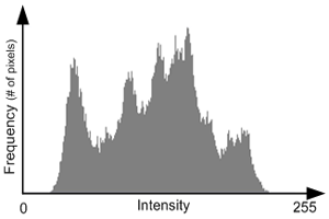
Histogram is a graphical representation of data distribution. Histogram is used to enhance the image contrast or to determine the threshold values.
Related Topics: Brightness, Contrast
Download: histoEqualization.zip
Histogram
In DSP, we store the number of pixels (frequencies) of same intensity values into a histogram array, which is commonly called "bin". For an 8-bit grayscale image, the size of histogram bin is 256, because the range of the intensity of 8-bit image is from 0 to 255.

Histogram is a useful tool to analyze the brightness and contrast of an image. It shows how the intensity values of an image is distributed and the range of brightness from dark to bright.
An image can be enhanced by remapping the intensity values using the histogram. Also, histogram is used to segmentize an image into the several regions by thresholding. For example, if the image intensities in the histogram are divided into 2 groups, the threshold value can be chosen at the middle of 2 peaks in the histogram.
Building a histogram of an image is quite easy. Traverse all pixels and count up the intensity values.
// traverse all pixels and accumulate the count of same intensity values
for ( i = 0; i < pixelCount; ++i )
{
    histogram[image[i]]++;
}
Histogram Equalization
Histogram equalization redistributes the pixel intensity values evenly by using cumulative(sum) histogram as a transfer function or as a look-up table.

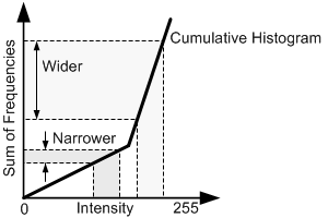
based on the slope of cumulative histogram.
The idea of histogram equalization comes from the cumulative histogram. Take a look at the left image of an example of cumulative histogram. The frequencies (the number of pixels) at each intensity value are accumulated. The higher pixel density is, the greater steepness is. There are 2 intervals with same width, but different slopes; one interval has slow steepness, and the other interval has steep slope. Let's project the intervals of the intensity values onto the other axis. Once they are projected, they have different intervals on the projected axis. If the slope is less than 1, the interval gets narrower. If the slope is greater than 1, then the interval is going to be wider. In other words, we are going to spread the intensity range if the pixel density is high, and shrink the interval if the density is low. Histogram equalization works best on an over or under exposed image, which has narrow contrast range.
In histogram equalization, the input pixel intensity, x is transformed to new intensity value, x′ by T. The transform function, T is the product of a cumulative histogram and a scale factor. The scale factor is needed to fit the new intensity value within the range of the intensity values, for example, 0 ~ 255.

The algorithm of cumulative histogram and histogram equalization look like this;
// build a cumulative histogram as LUT
for ( i=0; i < HISTOGRAM_SIZE; ++i )
{
    sum += histogram[i];
    sumHistogram[i] = sum;
}

// transform image using sum histogram as a LUT (Look Up Table)
for ( i = 0; i < pixelCount; ++i )
{
    outImage[i] = sumHistogram[image[i]] * MAX_INTENSITY / pixelCount;
}
The above code is not efficient because it does multiplication and division for every pixel. For faster computation, we can directly build a look up table by putting this product and division in it;
// build a LUT containing scale factor
for ( i=0; i < HISTOGRAM_SIZE; ++i )
{
    sum += histogram[i];
    lut[i] = sum * MAX_INTENSITY / pixelCount;
}

// transform image using sum histogram as a LUT
for ( i = 0; i < pixelCount; ++i )
{
    outImage[i] = lut[image[i]];
}
Examples
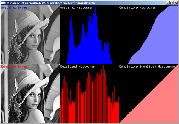
The following image is a screenshot of an example of histogram equalization, histoEqualization.zip.

Notice that the cumulative histogram after histogram equalization. It is almost linear, which means the number of intensity values are evenly distributed.
Download the source code and binary here: histoEqualization.zip