Window Filters
Related Topics: Convolution, Canny Edge Detection
Download: conv2d_edge.zip, conv2d_laplace.zip, conv2d_sharpen.zip
- Overview
- Smoothing Filter
- Edge Detection Filter
- Example: Edge Detection
- Laplacian Filter
- Example: Laplacian
- Sharpening Filter
- Example: Sharpen
Overview
Window filters are image processing operators to process a pixel with its neighbourhood pixels. The filters are used for computer vision and image processing such as filtering and edge detection. Window filters are mostly 2D kernels which are performing 2D convolution on the input image.
There are 2 major categories in the window filters; low-pass filter and high-pass filter. Low-pass filter is to remove fine noise (high frequency) from the input image. And, high-pass filter is to detect the edges because it allows to pass only rapid value changes (high frequency) in the image. Note that the sum of all elemements of a low-pass filter should be 1, because it conserves the original intensity after applying convolution. On the contrary, the sum of all elements of a high-pass filter is 0. If the center pixel has no difference than the other neighbourhood pixels, it should return 0 in a high-pass filter.
This page introduces 2D window filters (mostly 3x3 matrix) that are commoly used in image processing.
Smoothing Filters
Box (Average) Filter
Box filter is the simplest low-pass operator to smooth the input image. It is useful to remove high-frequency noise. It simply adds all pixels with the same weight and find the average value. As a result, the output image is getting blurry.

Gaussian Filter

Gaussian filter uses the standard normal distribution function to reduce high-frequency noise. It applys a higher weight at the center pixel and lesser weights while it is farther away. So, it produces more natural blur image than the box filter.


Here is a C++ code snippet to generate a 1D Gaussian kernel. The standard deviation, σ determines how the function is dispersed.
// make 1D gaussian kernel using normal distribution function
// do only half(positive area) and mirror to negative side
// because Gaussian is even function, symmetric to Y-axis
void generateGaussianKernel(float sigma, float *kernel, int kernelSize)
{
    float sum = 0;                 // used for normalization
    double result = 0;             // result of gaussian func

    int center = kernelSize / 2;   // center value of n-array(0 ~ n-1)

    if(sigma == 0)
    {
        for(int i = 0; i <= center; ++i)
            kernel[center+i] = kernel[center-i] = 0;

        kernel[center] = 1.0;
    }
    else
    {
        for(int i = 0; i <= center; ++i)
        {
            // dividing (sqrt(2*PI)*sigma) is not needed because normalizing result later
            result = exp(-(i*i)/(double)(2*sigma*sigma));
            kernel[center+i] = kernel[center-i] = (float)result;
            sum += (float)result;
            if(i != 0) sum += (float)result;
        }

        // normalize kernel
        // make sum of all elements in kernel to 1
        for(int i = 0; i <= center; ++i)
            kernel[center+i] = kernel[center-i] /= sum;
    }
}
Or, the gaussian filter can be also approximated with Pascal's triangle. The following is a 3x3, 5x5 and 7x7 Gaussian kernels using Pascal's triangle. Note that the gaussian kernel is seperable, so it can be performed 1D convolution twice; vertical and horizontal to reduce the mathematical computation. A 2D convolution with a 3x3 kernel requires 9 multiplications, however, a seperable convolution requires only 6 multiplications.


Please check WebGL version of Gaussian Blur implementation for more performance optimization using GLSL shaders.
Edge Detection Filters
Edge detection kernels are high-pass filters by finding the gradients in horizontal or vertical direction.

The horizontal gradient, Gx and vertical gradient, Gy can be approximated using the central difference.

To find the edges from the input image, first apply 2D convolution with Gx and Gy kernels to the input image. Then, compute the magnitude of the gradients because the gradient values are signed (can be negative). Higher magnitude value represents stronger edge.

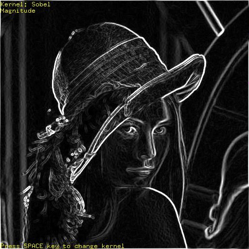
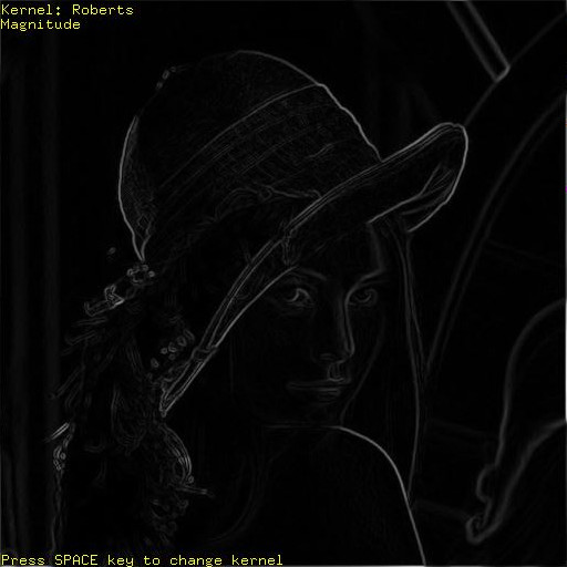
There are several variations of computing gradients; Prewitt, Sobel and Roberts operators. The magitude of each gradient operator follows. Notice that the edges lines are thicker (more than 1 pixel) and discontinuous. Canny Edge detection algorithm is thinning the edges with 1-pixel wide and connecting the discontinuous the edges togather.

Prewitt Filter
Prewitt edge detection operator uses equal weights in the gradient function.

Therefore, the 3x3 Prewitt gradient kernels Gx and Gy are;


Sobel Filter
Sobel edge detection operator uses a higher weight for the center pixel in the gradient functions. The 3x3 Gx and Gy of Sobel gradient kernels are;


Roberts Filter
Roberts gradient function uses diagonal neighbour pixels to calculate the difference. And, the gradient kernels are 2x2 matrix.

Example: Edge Detection
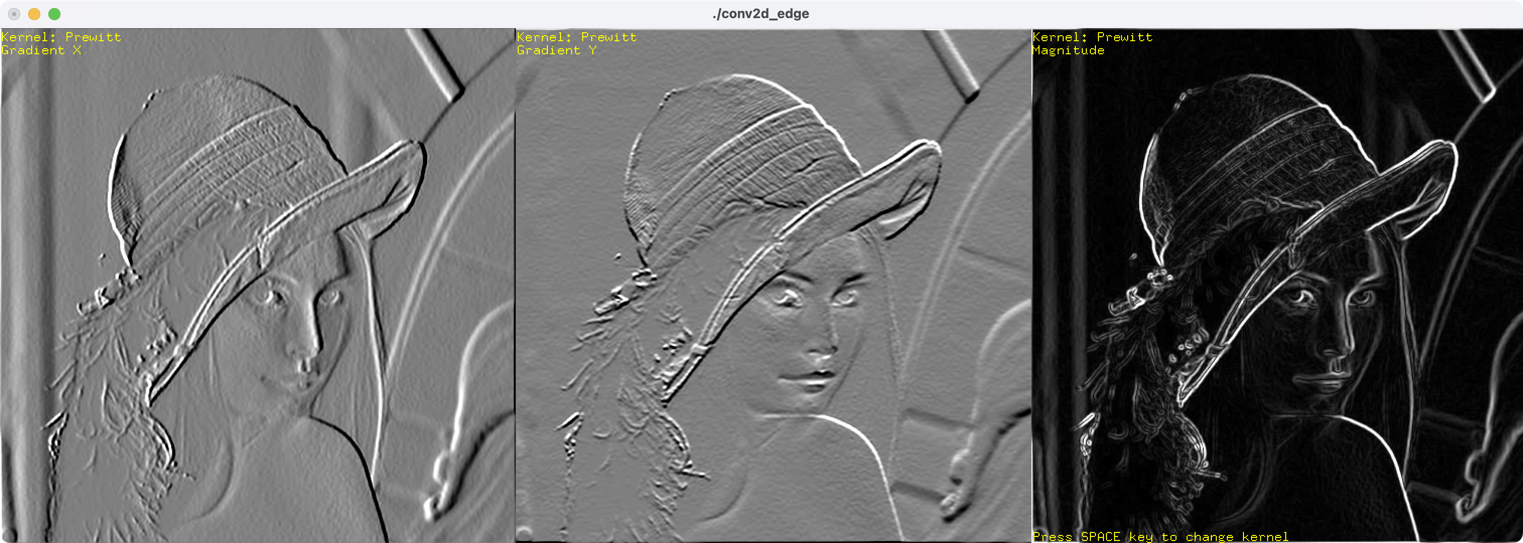
This C++ example calculates the gradients and magnitude of edge detection operators. Press SPACE key to switch the edge detection kernel; Prewitt, Sobel or Roberts.
Download: conv2d_edge.zip
Laplacian Filters
Laplacian kernel is a sum of second-order derivatives of horizontal and vertical directions to find edges from the input image, where zero crossings at the edges in the image.


The second-order gradients are computed by finding the central differences twice in horizontal or vertical directions. And, the 3x3 laplacian kernel can be written;


Example: Laplacian Kernel
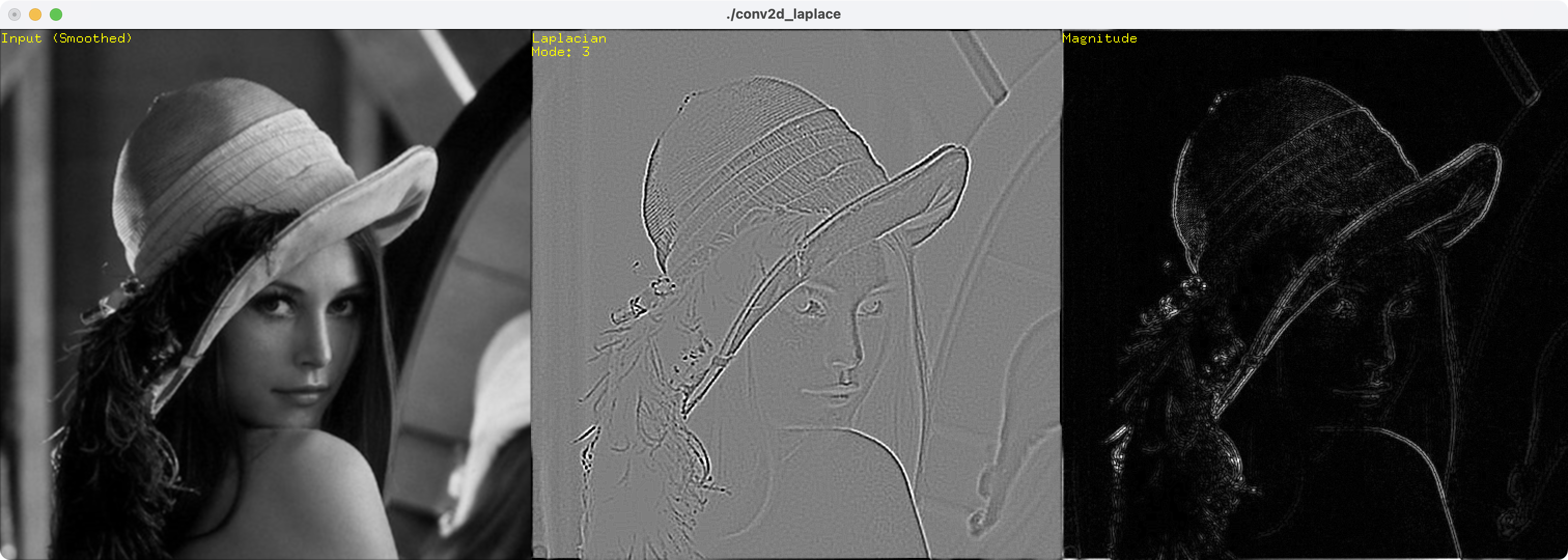
Download: conv2d_laplace.zip
This C++ example convoles the input image with 3x3 Laplacian kernel and computes its magnitude of the laplacian. Press SPACE key to switch the various laplacian kernels. Since Laplacian kernel is also a high-pass filter, the sum of the all elements should be 0.


Sharpening Filters
Unsharp Mask
If you subtract the smoothed image from the original image, you can get the details only which are the edges of the image. It is called unsharp mask.
Unsharp Mask = Original Image - Burred Image
By combining the original image and unsharp mask together, the resulting image produces clearer and enhances the edges and details in the original image. The following intensity profile diagrams show the steps of sharpening process using the unsharp mask.


Please see the sharpening example with a typical image.
Sharpening Kernel
The unsharp mask is similar to the result of applying the laplacian filter to the input image. The difference is the peaks of the intensity changes are inverted. Therefore, we can construct the sharpening kernel by subtracting the laplacian output from the input image.


Example: Sharpening

Download: conv2d_sharpen.zip
This C++ example enhances the image using various sharpening techniques. Press SPACE to change the filters.
- Mode 1: Adding the unsharp mask to the input image
- Mode 2: Subtracting the Laplacian from the input image
- Mode 3: Convolving the sharpening kernel
- Mode 4: Convolving the boost sharpening kernel (with diagonal)