Convolution

Convolution is the most important and fundamental concept in signal processing and analysis. By using convolution, we can construct the output of system for any arbitrary input signal, if we know the impulse response of system.

How is it possible that knowing only impulse response of system can determine the output for any given input signal? We will find out the meaning of convolution.

Related Topics: 2D Convolution Example, Proof of 2D Separable Convolution
Download: conv1d.zip, conv2d.zip

• Definition
• Impulse Function Decomposition
• Impulse Response
• Back to the Definition
• Convolution in 1D
• C++ Implementation for Convolution 1D
• Convolution in 2D
• Separable Convolution 2D
• C++ Algorithm for Convolution 2D

Definition

First, let's see the mathematical definition of convolution in discrete time domain. Later we will walk through what this equation tells us.
(We will discuss in discrete time domain only.)

where x[n] is input signal, h[n] is impulse response, and y[n] is output. * denotes convolution. Notice that we multiply the terms of x[k] by the terms of a time-shifted h[n] and add them up.

The keystone of understanding convolution is lying behind impulse response and impulse decomposition.

Impulse Function Decomposition

In order to understand the meaning of convolution, we are going to start from the concept of signal decomposition. The input signal is decomposed into simple additive components, and the system response of the input signal results in by adding the output of these components passed through the system.

In general, a signal can be decomposed as a weighted sum of basis signals. For example, in Fourier Series, any periodic signal (even rectangular pulse signal) can be represented by a sum of sine and cosine functions. But here, we use impulse (delta) functions for the basis signals, instead of sine and cosine.

Examine the following example how a signal is decomposed into a set of impulse (delta) functions. Since the impulse function, δ[n] is 1 at n=0, and zeros at n ≠ 0. x[0] can be written to 2·δ[n]. And, x[1] will be 3·δ[n-1], because δ[n-1] is 1 at n=1 and zeros at others. In same way, we can write x[2] by shifting δ[n] by 2, x[2] = 1·δ[n-2]. Therefore, the signal, x[n] can be represented by adding 3 shifted and scaled impulse functions.

In general, a signal can be written as sum of scaled and shifted delta functions;

Impulse Response

Impulse response is the output of a system resulting from an impulse function as input.
And it is denoted as h[n].

If the system is time-invariant, the response of a time-shifted impulse function is also shifted as same amount of time.

For example, the impulse response of δ[n-1] is h[n-1]. If we know the impulse response h[n], then we can immediately get the impulse response h[n-1] by shifting h[n] by +1. Consequently, h[n-2] results from shifting h[n] by +2.

If the system is linear (especially scalar rule), a scaled in input signal causes an identical scaling in the output signal.

For instance, the impulse response of 3·δ[n] is just multiplying by 3 to h[n].

If the input has 3 components, for example, a·δ[n] + b·δ[n-1] + c·δ[n-2], then the output is simply a·h[n] + b·h[n-1] + c·h[n-2]. This is called additive property of linear system, thus, it is valid only on the linear system.

Back to the Definition

By combining the properties of impulse response and impulse decomposition, we can finally construct the equation of convolution. In linear and time-invariant system, the response resulting from several inputs can be computed as the sum of the responses each input acting alone.

For example, if input signal is x[n] = 2·δ[n] + 3·δ[n-1] + 1·δ[n-2], then the output is simply y[n] = 2·h[n] + 3·h[n-1] + 1·h[n-2].

Therefore, we now clearly see that if the input signal is , then the output will be . Note one condition; convolution works on the linear and time invariant system.

To summarize, a signal is decomposed into a set of impulses and the output signal can be computed by adding the scaled and shifted impulse responses.

Furthermore, there is an important fact under convolution; the only thing we need to know about the system's characteristics is the impulse response of the system, h[n]. If we know a system's impulse response, then we can easily find out how the system reacts for any input signal.

Convolution in 1D

Let's start with an example of convolution of 1 dimensional signal, then find out how to implement into computer programming algorithm.

x[n] = { 3, 4, 5 }
h[n] = { 2, 1 }

x[n] has only non-zero values at n=0,1,2, and impulse response, h[n] is not zero at n=0,1. Others which are not listed are all zeros.

One thing to note before we move on: Try to figure out yourself how this system behaves, by only looking at the impulse response of the system. When the impulse signal is entered the system, the output of the system looks like amplifier and echoing. At the time is 0, the intensity was increased (amplified) by double and gradually decreased while the time is passed.

From the equation of convolution, the output signal y[n] will be .
Let's compute manually each value of y[0], y[1], y[2], y[3], ...

Notice that y[0] has only one component, x[0]h[0], and others are omitted, because others are all zeros at k ≠ 0. In other words, x[1]h[-1] = x[2]h[-2] = 0. The above equations also omit the terms if they are obviously zeros.

If n is larger than and equal to 4, y[n] will be zeros. So we stop here to compute y[n] and adding these 4 signals (y[0], y[1], y[2], y[3]) produces the output signal y[n] = {6, 11, 14, 5}.

Let's look more closely the each output. In order to see a pattern clearly, the order of addition is swapped. The last term comes first and the first term goes to the last. And, all zero terms are ignored.

y[0] = x[0]·h[0]
y[1] = x[1]·h[0] + x[0]·h[1]
y[2] = x[2]·h[0] + x[1]·h[1]
y[3] = x[3]·h[0] + x[2]·h[1]

Can you see the pattern? For example, y[2] is calculated from 2 input samples; x[2] and x[1], and 2 impulse response samples; h[0] and h[1]. The input sample starts from 2, which is same index as the sample point of output, and decreased. The impulse response sample index starts from 0 and increased.

Based on the pattern that we found, we can write an equation for any sample of the output;

where i is the index of any sample point and k is the number of samples in impulse response.

For instance, if an impulse response has 4 samples, the sample of output signal at index 9 is;
y[9] = x[9]·h[0] + x[8]·h[1] + x[7]·h[2] + x[6]·h[3]

Notice the first sample, y[0] has only one term. Based on the pattern that we found, y[0] is calculated as:
y[0] = x[0]·h[0] + x[-1]·h[1]. Because x[-1] is not defined, we simply pad it to zero.

C++ Implementation for Convolution 1D

Implementing the convolution algorithm is quite simple. The code snippet is following;

for ( i = 0; i < sampleCount; i++ )
{
    y[i] = 0;                       // set to zero before sum
    for ( j = 0; j < kernelCount; j++ )
    {
        y[i] += x[i - j] * h[j];    // convolve: multiply and accumulate
    }
}

However, you should concern several things in the implementation.
Watch out the range of input signal. You may be out of bound of input signal, for example, x[-1], x[-2], and so on. You can pad zeros for those undefined samples, or simply skip the convolution at the boundary. The results at the both the beginning and end edges cannot be accurate anyway.

Second, you need rounding the output values, if the output data type is integer and impulse response is floating point number. And, the output value may be exceeded the maximum or minimum value.
If you have unsigned 8-bit integer data type for output signal, the range of output should be between 0 and 255. You must check the value is greater than the minimum and less than the maximum value.

Download the 1D convolution routine and test program.
conv1d.zip

Convolution in 2D

2D convolution is just extension of previous 1D convolution by convolving both horizontal and vertical directions in 2 dimensional spatial domain. Convolution is frequently used for image processing, such as smoothing, sharpening, and edge detection of images.

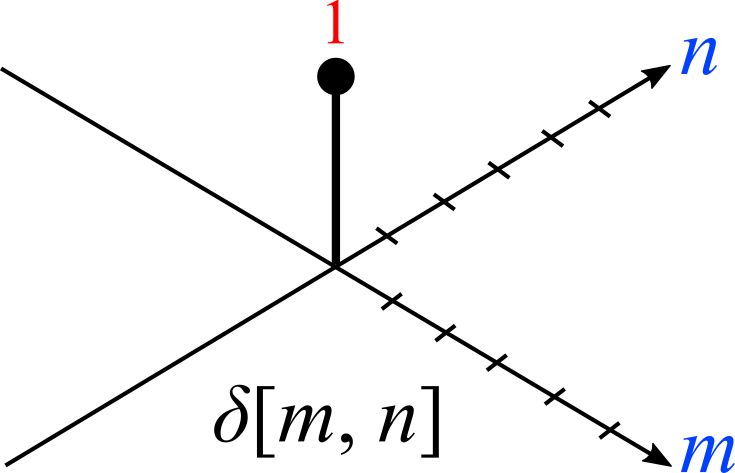
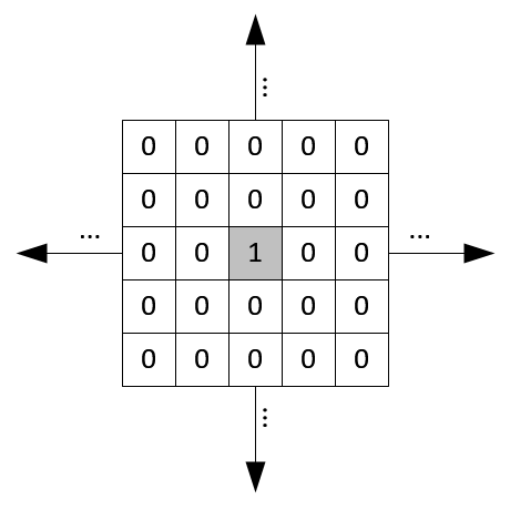
The impulse (delta) function is also in 2D space, so δ[m, n] has 1 where m and n is zero and zeros at m,n ≠ 0. The impulse response in 2D is usually called "kernel" or "filter" in image processing.

The second image is 2D matrix representation of impulse function. The shaded center point is the origin where m=n=0.

Once again, a signal can be decomposed into a sum of scaled and shifted impulse (delta) functions;

For example, x[0, 0] is x[0, 0]·δ[m, n], x[1, 2] is x[1, 2]·δ[m-1, n-2], and so on. Note that the matrices are referenced here as [column, row], not [row, column]. m is horizontal (column) direction and n is vertical (row) direction.

And, the output of linear and time invariant system can be written by convolution of input signal x[m, n], and impulse response, h[m, n];

Notice that the kernel (impulse response) in 2D is center originated in most cases, which means the center point of a kernel is h[0, 0]. For example, if the kernel size is 5, then the array index of 5 elements will be -2, -1, 0, 1, and 2. The origin is located at the middle of kernel.

Examine an example to clarify how to convolve in 2D space.
Let's say that the size of impulse response (kernel) is 3x3, and it's values are a, b, c, d,...

Notice the origin (0,0) is located in the center of the kernel.

Let's pick a simplest sample and compute convolution, for instance, the output at (1, 1) will be;

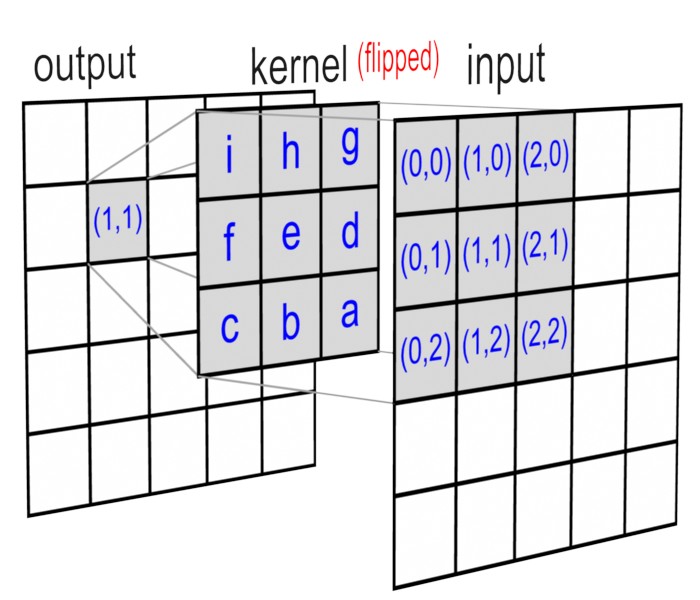
It results in sum of 9 elements of scaled and shifted impulse responses. The following image shows the graphical representation of 2D convolution.

Notice that the kernel matrix is flipped both horizontal and vertical direction before multiplying the overlapped input data, because x[0,0] is multiplied by the last sample of impulse response, h[1,1]. And x[2,2] is multiplied by the first sample, h[-1,-1].

Exercise a little more about 2D convolution with an another example. Suppose we have 3x3 input and 3x3 kernel matrices as follow.

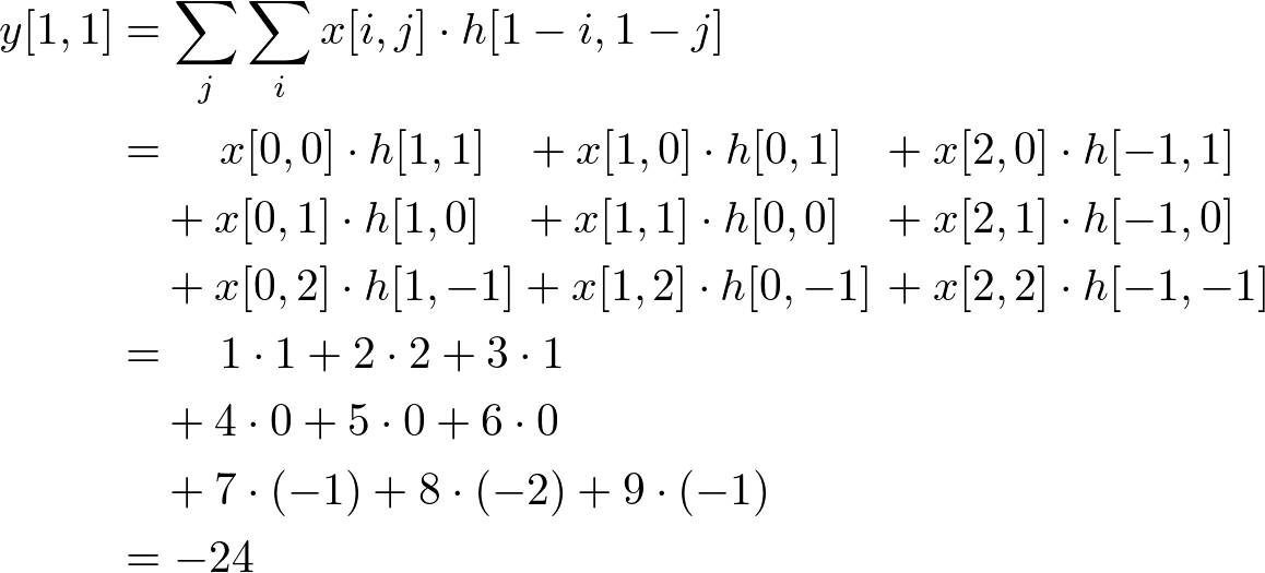
The ouput at (1, 1) for this example will be;

The complete solution for all 9 output can be found here; Example of 2D Convolution

Separable Convolution 2D

In convolution 2D with M×N kernel, it requires M×N multiplications for each sample. For example, if the kernel size is 3x3, then, 9 multiplications and accumulations are necessary for each sample. Thus, convolution 2D is very expensive to perform multiply and accumulate operation.

However, if the kernel is separable, then the computation can be reduced to M + N multiplications.

A matrix is separable if it can be decomposed into (M×1) and (1×N) matrices.
For example;

And, convolution with this separable kernel is equivalent to;

(Proof of Separable Convolution 2D)

As a result, in order to reduce the computation, we perform 1D convolution twice instead of 2D convolution; convolve with the input and M×1 kernel in vertical direction, then convolve again horizontal direction with the result from the previous convolution and 1×N kernel. The first vertical 1D convolution requires M times of multiplications and the horizontal convolution needs N times of multiplications, altogether, M+N products.

However, the separable 2D convolution requires additional storage (buffer) to keep intermediate computations. That is, if you do vertical 1D convolution first, you must preserve the results in a temporary buffer in order to use them for horizontal convolution subsequently.

Notice that convolution is associative; the result is same, even if the order of convolution is changed. So, you may convolve horizontal direction first then vertical direction later.

Gaussian smoothing filter is a well-known separable matrix. For example, 3x3 Gaussian filter is;

C++ Algorithm for Convolution 2D

We need 4 nested loops for 2D convolution instead of 2 loops in 1D convolution.

// find center position of kernel (half of kernel size)
kCenterX = kCols / 2;
kCenterY = kRows / 2;

for(i=0; i < rows; ++i)              // rows
{
    for(j=0; j < cols; ++j)          // columns
    {
        for(m=0; m < kRows; ++m)     // kernel rows
        {
            mm = kRows - 1 - m;      // row index of flipped kernel

            for(n=0; n < kCols; ++n) // kernel columns
            {
                nn = kCols - 1 - n;  // column index of flipped kernel

                // index of input signal, used for checking boundary
                ii = i + (kCenterY - mm);
                jj = j + (kCenterX - nn);

                // ignore input samples which are out of bound
                if( ii >= 0 && ii < rows && jj >= 0 && jj < cols )
                    out[i][j] += in[ii][jj] * kernel[mm][nn];
            }
        }
    }
}

The above snippet code is simple and easiest way to understand how convolution works in 2D. But it may be the slowest implementation.

Take a look at a real example; convolution with 256x256 image and 5x5 Gaussian filter.

The source image is uncompressed raw, 8-bit (unsigned char) grayscale image. And again, Gaussian kernel is separable;

On my system (Intel i7-7700HQ 2.8GHz), normal convolution took about 5.1 ms and separable convolution took only 1.8 ms. You can see how much separable convolution is faster compared to normal 2D convolution.

Download 2D convolution application and source code here: conv2d.zip (updated 2018-06-28)
The program uses OpenGL to render images on the screen.