Proof of Separable Convolution 2D

By the definition of Convolution 2D;

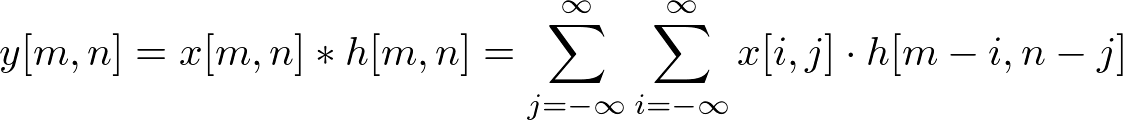
Since convolution is commutative (x[n] * h[n] = h[n] * x[n]), swap the order of convolution;

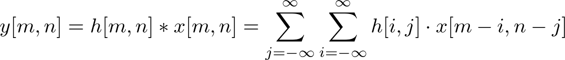
And, if h[m, n] is separable to (M×1) and (1×N);

Therefore, substitute h[m, n] into the equation;

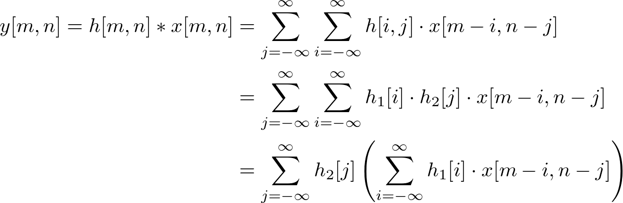
Since the definition of convolution 1D is;

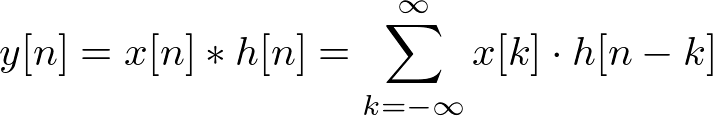
it is convolving with input and h₁, then convolve once again with the result of previous convolution and h₂. Therefore, the separable 2D convolution is performing twice of 1D convolution in horizontal and vertical direction.

And, convolution is associative, it does not matter which direction perform first. Therefore, you can convolve with h₂[n] first then convolve with h₁[m] later.

Example

Compute y[1,1] by using separable convolution method and compare the result with the output of normal convolution 2D.

i) Using convolution 2D

ii) Using Separable Convolution 2D
First, do the vertical convolution 1D where the row is n=1, and the column is m=0,1,2;


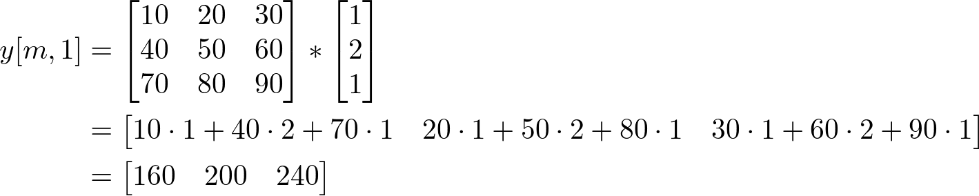
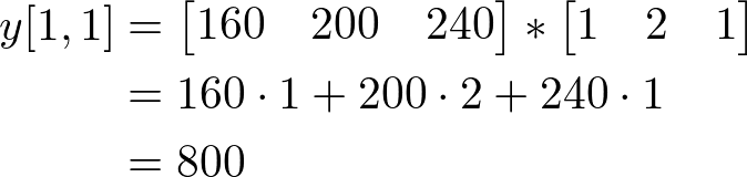
Then, do the horizontal convolution with above result where column is m=1;

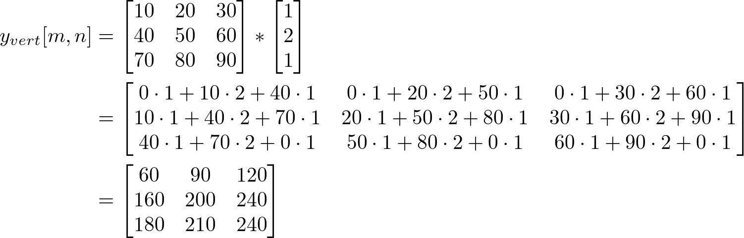
You may not see the benefit of separable convolution if you do seperable convolution for only 1 sample. It looks like more multiplications needed than regular 2D convolution does. Here is the full separable convolution for all 9 input data at once. First, perform the vertical convolution for the input signal and store the interim result to y_vert[m,n].

Then, perform the horizontal convolution on y_vert[m,n] to find the final output signal, y[m,n].

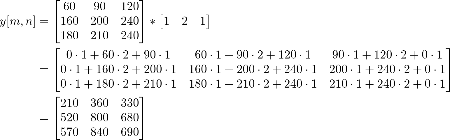
Since the kernal size is 3x3, the regular 2D convolution requires 9 multiplications and 9 additions per sample. However, using seperable convolution, each sample requires only 6 multiplications (3 for vertical and 3 for horizontal convolution) and 4 additions.